Jeongwoo Park (MSc Data Science, 2023)
Ⅰ. The Digital Advertising Market is Facing the Issue of Measurement Error
Digital advertising has been growing explosively every year. Especially during the global pandemic, as the offline market significantly contracted, the shift in consumer focus to online platforms made digital advertising the mainstream in the global advertising market.
The core of digital advertising is undoubtedly the smartphone. With the ability to access the web anytime and anywhere via smartphones, internet-based media have emerged in the advertising market. Particularly, app-based platform services that offer customized user experiences have surged rapidly, significantly contributing to the growth of digital advertising. This market has been driven by the convenience smartphones offer compared to traditional devices like PCs and tablets.
However, the digital advertising industry is currently grappling with the issue of "Measurement Error". This problem causes significant disruptions in accurately measuring and predicting advertising performance.
The rapidly growing digital advertising market
The key difference between digital advertising and traditional advertising is the ability to track results. In traditional advertising, companies could only estimate performance by saying, "I advertised on a platform seen by thousands of people per day" to gauge brand awareness. As a result, even when advertising agencies tried to analyze performance, they often faced dissatisfaction due to the difficulty in accurately assessing outcomes because of various types of noise.
With the advent of the web, advertising entered a new phase. Information of users is stored in cookies when they access websites, allowing advertisers to instantly track which ads users viewed, which products they looked at, and what they purchased. As a result, companies can now easily verify how effective their ads are on users. Furthermore, they can compare multiple ads and quickly determine the direction for planning future campaigns.
The advent of smartphones has accelerated this paradigm shift. Unlike in the past when multiple people shared a single PC or tablet, we are now in the era of "one person, one smartphone", allowing behavior patterns on specific devices to be attributed to individual users. In fact, according to a 2022 Gallup Korea survey, the smartphone penetration rate among Korean adults was 97%. In recent years, many companies have introduced hyper-personalized tareting services to the public, signaling a major shift in the digital advertising market.
Issue in Digital Advertising: Measurement Error
However, everything has its pros and cons, and digital advertising is no exception. Industry professionals point out that the effectiveness of digital ads is hindered by factors such as user fatigue and privacy concerns. From my own experience in the advertising industry, the issue that stands out the most is "measurement error".
Measurement error refers to data being distorted due to specific factors, resulting in outcomes that differ from the true values. Common issues in the industry include users being exposed to the same ad multiple times in a short period, leading to insignificant responses, or fraudulent activities where malicious actors create fake ad interactions to gain financial benefits. Additionally, technical problems such as server instability can cause user data to be double counted, omitted, or delayed. For various reasons, the data becomes "contaminated", preventing advertisers from accurately assessing ad performance.
Of course, media companies that deliver the ads are not idle either. They continuously update advertising reports, correcting inaccurate data related to ad spend, impressions, clicks, and other performance metrics. During this process, advertisers change the reported ad performance for up to one week.
The problem is that for "demanders" like me, for whom accurate measurement of ad performance is crucial, measurement error leads to an endogeneity issue in performance analysis, significantly reducing the reliability of the analysis. Simply put, because the reports keep being revised due to measurement errors, it becomes difficult to accurately analyze ad performance.
Even in the advertising industry, where the focus is not on performance measurement but on predicting future values, the issue of measurement error remains significant. This is because measurement error increases the variance of the residuals, reducing the model's goodness of fit. Additionally, in cases where the magnitude of the measurement error changes daily due to the frequency of data updates, as with digital advertising data, non-linear models that do not guarantee linearity are more likely to show poor predictive performance in extrapolation.
Unfortunately, due to the immediacy characteristic of digital advertising, advertisers cannot afford to wait up to a week for the data to be fully updated. If advertisers judge that an ad's performance is poor, they may immediately reduce its exposure or even stop the campaign altogether. Additionally, for short-term ads, such as promotions, waiting up to a week is not an option.
The situation is no different for companies claiming to use "AI" to automatically manage ads. Advertising automation is akin to solving a reinforcement learning problem, where the goal is to maximize overall ad performance within a specific period using a limited budget. When measurement error occurs in the data, it can disrupt the initial budget allocation. Ultimately, it is quite likely to result in optimization failure.
Research Objective: Analysis of the Impact of Measurement Error and Proposal of a Reasonable Prediction Model
If, based on everything we've discussed so far, you're thinking, "The issue of measurement error could be important in digital advertising," then I've succeeded. Unfortunately, the advertising industry is not paying enough attention to measurement error. This is largely because measurement errors are not immediately visible.
This article focuses on two key aspects. First, we analyzed the impact of measurement error on advertising data based on the size of the measurement error and the data. Second, we proposed a reasonable prediction model that considers the characteristics of the data.
II. Measurement Error from a Predictive Perspective
In this chapter, we will examine how measurement error affects actual ad performance.
Measurement Error: Systematic Error and Random Error
Let's delve a bit deeper into measurement error. Measurement error can be divided into two types: systematic error and random error. Systematic error has a certain directionality; for example, values are consistently measured higher than the true value. This is sometimes referred to as the error having a "drift". On the other hand, random error refers to when the measured values are determined randomly around the true value.
So, what kind of distribution do the measured values follow? For instance, if we denote the size of the drift as $\alpha$ and the true value as $\mu$, the measured value, represented as the random variable X, can be statistically modeled as following a normal distribution, $N(\mu + \alpha, \sigma^{2})$. In other words, the measured value is shifted by $\alpha$ from the true value (systematic error) while also having variability of $\sigma^2$ (random error).
Systematic errors can be resolved through data preprocessing and scaling, so they are not a significant issue from an analyst's perspective. Specifically, removing the directional bias by $\alpha$ from the measurements is usually sufficient. On the other hand, random errors significantly influence the magnitude of measurement errors and can cause problems. To resolve this, a more statistically sophisticated approach is required from the analyst's perspective.
Let's take a closer look at the issues that occur when data contains random errors. In regression models, when measurement errors are included in the independent variables, a phenomenon known as "Regression Dilution" occurs, where the absolute value of the estimated regression coefficients shrinks towards zero. To understand this better, imagine including an independent variable filled with measurement errors in the regression equation. Since this variable fluctuates randomly due to the random component, the effect of the regression coefficient will naturally appear as zero. This issue is not limited to basic linear regression models but occurs in all linear and nonlinear models.
The Data Environment in Digital Advertising
So far, we have discussed measurement errors. Now, let's examine the environment in which digital advertising data is received for modeling purposes. In Chapter 1, we mentioned that media companies continuously update performance data such as impressions, clicks, and ad spend to address measurement errors. Given that the data is updated up to a week later, when the data is first received, it is likely that a significant amount of measurement error is present. However, as the data gets updated the next day, it becomes more accurate, and by the following day, it becomes even more precise. Through this process, the measurement error in the data tends to decrease exponentially.
Since the magnitude of measurement errors changes with each update, this can lead to issues of heteroskedasticity in addition to model fit. When heteroskedasticity occurs, the estimates become inefficient from an analytic perspective. Furthermore, from a predictive perspective, it presents challenges for extrapolation, as predicting new values based on existing data tends to result in poor performance.
Additionally, as ad spend increases, the magnitude of measurement errors grows. For example, when spending 1 dollar on advertising, the measurement error might only be a few cents, but with an ad spend of 1 million dollars, the error could be tens of thousands of dollars. In this context, it makes sense to use a multiplicative model, where a random percentage change is applied based on the ad spend. Of course, it is well-known that regression dilution can occur in multiplicative models, just as it does in additive models.
Model and Variable Selection
We have defined the dependent variable as the "number of events" that occur after users respond to an ad, based on their actions on the web or app. Events such as participation, sign-ups, and purchases are countable, occurring as 0, 1, 2, and so on, which means a model that best captures the characteristics of count data is needed.
For the independent variables, we will use only "ad spend" and the "lag of ad spend," as these are factors that the advertiser can control. Metrics like impressions and clicks are variables that can only be observed after the ads have been served, meaning they cannot be controlled in advance, and are therefore excluded from a business perspective. Impressions are highly correlated with ad spend, meaning these two variables contain similar amounts of information. This will play an important role later in the modeling process.
Meanwhile, to understand the effect of measurement errors, we need to deliberately "contaminate" the data by introducing measurement errors into the ad spend. The magnitude of these errors was set within the typical range observed in the industry, and simulations were conducted across various scenarios.
The proposed models are a Poisson regression-based time series model and a Poisson Kalman filter. We chose models based on the Poisson distribution to reflect the characteristics of count data.
The reason for using Poisson regression is that it helps to avoid the issue of heteroskedasticity in the residuals. Due to the nature of Poisson regression and other generalized linear models (GLMs), the focus is on the relationship between the mean and variance through the link function. This allows us to mitigate the heteroskedasticity problem mentioned earlier to some extent.
Furthermore, using the Poisson Kalman filter allows us to partially avoid the measurement error issue. This model accounts for the Poisson distribution in the observation equation while also compensating for the inaccuracies (including measurement errors) in the observation equation through the state equation. This characteristic enables the model to inherently address the inaccuracies in the observed data.
The Effect of Measurement Error
First, we will assess the effect of measurement error using the Poisson time series model.
[ \log(\lambda{t}) = \beta{0} + \sum{k=1}^{7}\beta{k}\log(Y{t-k} + 1) + \alpha{7}\log(\lambda{t-7}) + \sum{i=1}^{8}\eta{i} Spend{(t-i+1)} ]
Here, Spend represents the ad spend from the current time point up to 7 time points prior, and $\beta$ captures the lagged effects embedded in the residuals, beyond the effect of ad spend. Additionally, $\alpha$ accounts for the day-of-week effects.

Although it may be too lengthy to include, we confirmed that this model reasonably reflects the data when considering model fit and complexity.
What we are really interested in is the measurement error. How did the measurement error affect the model’s predictions? To explore this, we first need to understand time series cross-validation.
Typically, K-fold or LOO (Leave-One-Out) methods are used when performing cross-validation on data. However, for time series data, where the order of the data is crucial, excluding certain portions of the data is not reasonable. Therefore, the following method is applied instead.
- Fit the model using the first $d$ data points and predict future values.
- Add one more data point, fit the model with ($d+1$) data points, and predict future values.
- Repeat this process.
This can be illustrated as follows.
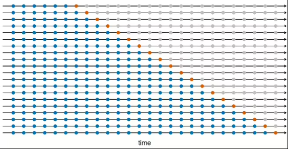
Using this cross-validation method, we calculated the 1-step ahead forecast accuracy, with the evaluation metric set as MAE (Mean Absolute Error), taking the Poisson distribution into account.

An interesting result was found: in the table above, for low levels of measurement error (0.5 ~ 0.7), the model with measurement error recorded a lower MAE than the model without it. Wouldn’t we expect the model without measurement error to perform better, according to conventional wisdom?
This phenomenon occurred due to the regularization effect introduced by the measurement error. In other words, the measurement error caused attenuation bias in the regression coefficients, which helped mitigate the issue of high variance to some extent. In this case, the measurement error effectively played the role of the regularization parameter, $\lambda$, that we typically focus on in regularization.
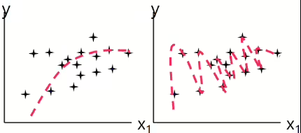

Let's look at Figure 5. If the variance of the measurement error increases infinitely, the variable becomes useless, as shown in the right-hand diagram. In this case, the model would be fitted only to the sample mean of the dependent variable, with an R-squared value of 0. However, we also know that a model with no regularization at all, as depicted in the left-hand diagram, is not ideal either. Ultimately, finding the right balance is crucial, and it’s important to “listen to the data” to achieve this.
Let’s return to the model results. While low levels of measurement error clearly provide an advantage from the perspective of MAE, higher levels of measurement error result in a higher MAE compared to the original data. Additionally, since measurement errors only occur in recent data, as the amount of data increases, the proportion of error-free data compared to data with measurement error grows, reducing the overall effect of the measurement error.
What does it mean that MAE gradually improves as the data size increases? Initially, the model had high variance due to its complexity, but as more data becomes available, the model begins to better explain the data.
In summary, a small amount of measurement error can be beneficial from the perspective of MAE, which means that measurement error isn’t inherently bad. However, since we can't predetermine the magnitude of measurement error in the independent variables, it can be challenging to decide whether a model that resolves the measurement error issue is better or if it's preferable to leave the error unresolved.
To determine whether stronger regularization would be beneficial, one approach is to add a constraint term with $\lambda$ to the model for testing. Since the measurement error has acted similarly to ridge regression, it is appropriate to test using L2 regularization in this case as well.
If weaker regularization is needed, what would be the best approach? In this case, one option would be to reduce measurement error by incorporating the latest data updates from the media companies. Alternatively, data preprocessing techniques, such as applying ideas from repeated measures ANOVA, could be used to minimize the magnitude of the measurement error.
III. Measurement Error from an Analytic Perspective
In Chapter 2, we explained that from a predictive perspective, an appropriate level of measurement error can act as regularization and be beneficial. At first glance, this might make measurement error seem like a trivial issue. But is that really the case?
In this chapter, we will explore how measurement error impacts the prediction of advertising performance from an analytic perspective.
Endogeneity: Disrupting Performance Measurement
In Chapter 1, we briefly discussed ad automation. Since a customer's ad budget is limited, the key to maximizing performance with a limited budget lies in solving the optimization problem of how much budget to allocate to each medium and ad. This decision ultimately determines the success of an automated ad management business.
There are countless media platforms and partners that play similar roles. It's rare for someone to purchase a product after encountering just one ad on a single platform. For example, consider buying a pair of pants. You might first discover a particular brand on Instagram, then search for that brand on Naver or Google before visiting a shopping site. Naturally, Instagram, Naver, and Google all contributed to the purchase. But how much did each platform contribute? To quantify this, the advertising industry employs various methodologies. One of the most prominent techniques is Marketing Media Mix Modeling.
As mentioned earlier, many models are used in the advertising industry, but the fundamental idea remains the same: distributing performance based on the influence of coefficients in regression analysis. However, the issue of "endogeneity" often arises, preventing accurate calculation of these coefficients. Endogeneity occurs when there is a non-zero correlation between the explanatory variables and the error term in a linear model, making the estimated regression coefficients unreliable. Accurately measuring the size of these coefficients is crucial for determining each platform's contribution and for properly building performance optimization algorithms. Therefore, addressing the issue of endogeneity is essential.
Solution to the Endogeneity Problem: 2SLS
In econometrics, a common solution to the endogeneity problem is the use of 2SLS (Two-Stage Least Squares). 2SLS is a methodology that addresses endogeneity by using instrumental variables (IV) that are highly correlated with the endogenous variables but uncorrelated with the model’s error term.
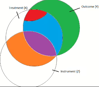
Let's take a look at the example in Figure 6. We are using independent variable X to explain the dependent variable Y, but there is endogeneity in the red section of X, which negatively affects the estimation. To address this, we can use an appropriate instrumental variable Z, which is uncorrelated with the residuals of Y after removing X's influence (green), ensuring validity, and correlated with the original variable X, ensuring relevance. By performing the regression analysis only on the intersection of Z and X (yellow + purple), we can explain Y while solving the endogeneity problem in X. The key idea behind instrumental variables is to sacrifice some models fit in order to remove the problematic (red) section.
Returning to the main point, in our model, there is not only the issue of measurement error in the variables, but also the potential for endogeneity due to omitted variable bias (OVB), as we are using only "ad spend" and lag variables as explanatory variables. Since the goal of this study is to understand the effect of measurement error on advertising performance, we will use a 2SLS test with appropriate IV to examine whether the measurement error in our model is actually causing endogeneity from an analytic perspective.
IV for Ad Spend: Impressions
As we discussed earlier, instrumental variables can help resolve endogeneity. However, verifying whether an instrumental variable is appropriate is not always straightforward. While it may not be perfect, for this model, based on industry domain knowledge, we have selected "impressions" as the most suitable instrumental variable.
First, let’s examine whether impressions satisfy the relevance condition. In display advertising, such as banners and videos, a CPM (cost per thousand impressions) model is commonly used, where advertisers are charged based on the number of impressions. Since advertisers are billed just for showing the ad, there is naturally a very high correlation between ad spend and impressions. In fact, a simple correlation analysis shows a correlation coefficient of over 0.9. This indicates that impressions and ad spend have very similar explanatory power, thus satisfying the relevance condition.
The most difficult aspect to prove for an instrumental variable is its validity. Validity means that the instrumental variable must be uncorrelated with the residuals, those are the factors in the dependent variable (advertising performance) that remain after removing the effect of ad spend. In our model, what factors might be included in the residuals? From a domain perspective, possible factors include the presence of promotions or brand awareness. Unlike search ads, where users actively search for products or brands, in display ads, users are passively exposed to ads, as advertisers pay to have them shown by the media platforms. Therefore, the number of impressions, which reflects forced exposure to ads, is likely uncorrelated with factors such as brand awareness or the presence of promotions, which influence the residuals.
If you're still uncertain about whether the validity condition is satisfied, you can perform a correlation test between the instrumental variable and the residuals. As shown in the results of Figure 7, we cannot reject the null hypothesis of no correlation at the significance level of 0.05.

Of course, the instrumental variable, impressions, also contains measurement error. However, it is known that while measurement error in the instrumental variable can reduce the correlation with the original variable, it does not affect its validity.
Method for Detecting Endogeneity: Durbin-Wu-Hausman Test
Now, based on the instrumental variable(impressions) we identified let’s examine whether measurement error affects the endogeneity of the coefficients. After performing the Durbin-Wu-Hausman test, we can see that in some intervals, the null hypothesis of no endogeneity is rejected. This indicates that the measurement error in the coefficients is indeed affecting endogeneity.

Depending on the patterns in the newly acquired data revealed through this test, even seemingly robust models can change. Therefore, we can conclude that modeling with consideration for measurement error is a safer approach.
IV. Poisson Kalman Filter and Ensemble
Up until now, we have explored measurement error from both predictive and analytic perspectives. This time, we will look into the Poisson Kalman Filter, which corrects for measurement error, and introduce an "ensemble" model that combines the Poisson Kalman Filter with the Poisson time series model.
Poisson Kalman Filter, Measurement Error, Bayesian, and Regularization
The Kalman filter is a model that finds a compromise between the information from variables that the researcher already knows (State Equation) and the actual observed values (Observation Equation). From a Bayesian perspective, this is similar to combining the researcher's prior knowledge (Prior) with the likelihood obtained from the data.
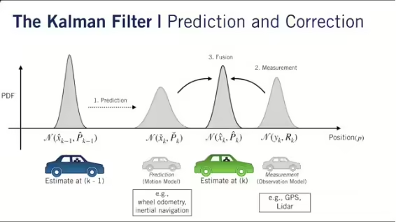
The regularization and measurement error introduced in Chapter 3 can also be interpreted from a Bayesian perspective. This is because the core idea of regularization aligns with how strongly we hold the prior belief in Bayesian modeling that $\beta=0$. In Chapter 3, we effectively drove the (random) measurement error coefficients toward zero, which ties together the intuition behind Kalman filters, Bayesian inference, regularization, and measurement error. Therefore, using a Kalman filter essentially means incorporating measurement error through the state equation, and this can further be understood as including regularization into the model.
Then, how should we construct the observation equation? Since our dependent variable is count data, it would be reasonable to use the log-link function from the GLM framework to model it effectively.
Poisson Time Series vs. Poisson Kalman Filter

Let’s compare the performance of the Poisson time series model and the Poisson Kalman filter. First, looking at the log likelihood, we can see that the Poisson time series model consistently has a higher value across all intervals. However, when we examine the MAE, the Poisson Kalman filter shows superior performance. This suggests that the Poisson time series model is overfitted compared to the Poisson Kalman filter. In terms of computation time, the Poisson Kalman filter is also faster. However, since both models take less than 2 seconds to compute, this is not a significant factor when considering their application in real-world services.
If you look closely at Figure 10, you can spot an interesting detail: the decrease in MAE as the data volume increases is significantly larger for the Poisson time series model compared to the Poisson Kalman filter. The reason for this is as follows.
The Poisson Kalman filter initially reflected the state equation well, leading to a significant advantage in prediction accuracy (MAE) early on. However, as more data was added, it seems that the observation equation failed to effectively incorporate the new data, resulting in a slower improvement in MAE. On the other hand, the Poisson time series model suffered from poor prediction accuracy early on due to overfitting, but as more data came in, it was able to reasonably incorporate the data, leading to a substantial improvement in MAE.
Similar results were found in the model robustness tests. Specifically, in tests for residual autocorrelation, mean-variance relationships, and normality, the Poisson Kalman filter performed better when there was a smaller amount of data early on. However, after the mid-point, the Poisson time series model outperformed it.
Ensemble: Combining the Poisson Time Series and the Poisson Kalman Filter
Based on the discussion so far, we have combined the distinct advantages of both models to build a single ensemble model.
To simultaneously account for bias and variance, we set the constraint for the stacked model, which minimizes MAE, as follows.
[ p{t+1} = argmin{p}\sum{i=1}^{t}w{i}|y{i} – (p * \hat{y}{i}^{(GLM)} + (1 – p) * \hat{y}_{i}^{(KF)})| ]
[ s.t. 0 \leq p \leq 1, \forall w > 0 ]
As we observed earlier, the Poisson Kalman filter had a lower MAE across all intervals, so without considering the momentum of MAE improvement, the stacked model would output $p=0$ across all intervals, meaning it would rely 100% on the Poisson Kalman filter. However, since the MAE of the Poisson time series model improves significantly in the later stages with a larger data set, we introduced a weight $W$ in front of the absolute constraint to account for this.
How should the weights be assigned? First, as the amount of data increases, both models will become progressively more reliable, resulting in reduced variance. Additionally, the model that performs better will typically have lower variance. Therefore, by assigning weights inversely proportional to the variance, we can effectively reflect the models' increasing accuracy over time.
The predictions from the final model, which incorporates the weights, are as follows.
[ \hat{y}{t+1} = p{t+1}\hat{y}{t+1}^{(GLM)} + (1 – p{t+1})\hat{y}_{t+1}^{(KF)} ]
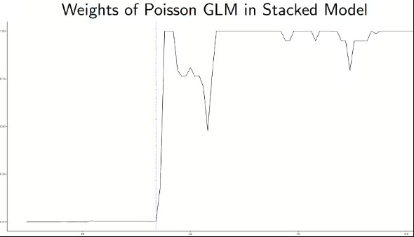
When analyzing the data using the ensemble model, we observed that in the early stages, p (the weight of the Poisson time series model in the ensemble) remained close to 0, but then jumped near 1 in the mid stages. Additionally, in certain intervals during the later stages where the data patterns change, we can see that the Poisson Kalman filter, which leverages the advantages of the state equation, is also utilized.

Let’s take a look at the MAE of the ensemble model in Figure 12. By reasonably combining the two models that exhibit heterogeneity, we can see that the MAE is lower across all intervals compared to the individual models. Additionally, in the robustness tests, we confirmed that the advantages of the ensemble were maximized, making it more robust than the individual models.
Conclusion
While the fields of applied statistics, econometrics, machine learning, and data science may have different areas of focus and unique strengths, they ultimately converge on the common question: "How can we rationally quantify real-world problems?" Additionally, a deep understanding of the domain to which the problem belongs is essential in this process.
This study focuses on the measurement error issues commonly encountered in the digital advertising domain and how these issues can impact both predictive and analytic modeling. To address this, we presented two models, the Poisson time series model and the Poisson Kalman filter, tailored to the domain environment (advertising industry) and the data generating process (DGP). Considering the strong heterogeneity between the two models, we ultimately proposed an ensemble model.
With the universalization of smartphones, the digital advertising market is set to grow even more rapidly in the future. I hope that as you read this paper, you take the time to savor the knowledge rather than hurriedly trying to absorb the text. It would be wonderful if you could expand your understanding of how statistics applies to the fields of data science and artificial intelligence.